The Bitcoin OTC Trust Network

Try it

Break the network yourself

Remove users and see what is left. Random failures take users at random; a targeted attack removes the most-connected users first. Blue users can still reach one another through the network; grey users have been cut off.

The measures

A sparse small world

We turned the ratings into a network: users are nodes, and a positive rating from one user to another is a directed link. Most classic network models are for undirected networks, so we also join two users with one link when either rated the other, which gives 18,591 links among 5,881 users. These are its basic measures.

Measure	Value	What it says
Average degree \(\langle k\rangle = 2L/N\)	6.32	Links per user; the largest hub has 788
Density \(2L/N(N-1)\)	0.11%	Very sparse: almost no pairs are linked
Average clustering \(\langle C\rangle\)	0.155	How often two neighbours of a user are also linked
Transitivity	0.057	Three times the triangles, divided by connected triples
Largest component	94.4%	Users who can reach each other
Mean distance \(\langle d\rangle\)	3.76	Links on a shortest path, inside the largest component
Diameter	14	The longest shortest path
Modularity	0.504	Strong community structure

Paths are shorter than in a random network of the same size, while clustering is about 150 times higher: together that is a small world. All five largest communities are weak communities in the sense of Barabási's Network Science, with more of their members' link ends inside the group than outside, although which users land in which group changes when the algorithm is rerun.

The models

What theory gets right, and wrong

We set the network beside three references: an Erdős–Rényi random network with the same users and links, a Barabási–Albert network grown by preferential attachment, and a degree-preserving randomization that keeps every user's degree but shuffles who is linked to whom.

	Observed	ER	BA	Rewired
Largest degree	788	17	231	788
Average clustering	0.155	0.001	0.008	0.061
Mean distance	3.76	4.91	4.08	3.52
Modularity	0.504	0.369	0.388	0.334

Keeping the degrees reproduces the short paths but not the clustering or the communities. Those come from how users actually chose their partners.

Heavy-tailed, but not strictly scale-free

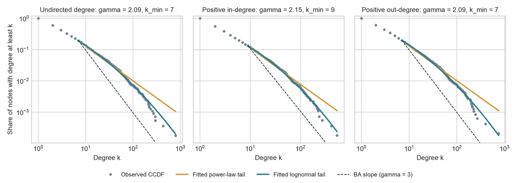
A scale-free network has a degree distribution \(P(k) \propto k^{-\gamma}\). Fitted properly, by maximum likelihood rather than a straight line on a log–log plot, the tail gives \(\gamma = 2.09\): heavier than the \(\gamma = 3\) of the BA model. Yet a lognormal tail fits better, and above about 100 links the data bend down.

BA's growth rule also fails, because 70.5% of links join two users who were already present. Barabási's internal-link model allows exactly that, and for the measured \(m = 0.99\) new and \(n = 2.35\) internal links per new user it predicts a value inside the fitted range:

Hubs and the structural cutoff

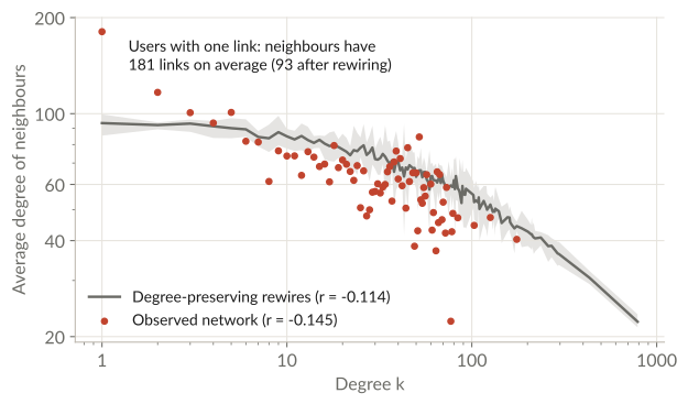
The negative assortativity is partly forced. In a simple network a hub cannot find enough other hubs to link to, and above the structural cutoff \(k_s = \sqrt{\langle k\rangle N} \approx 193\) that alone pushes \(r\) below zero. Randomizations that keep every degree already give \(r = -0.114\). The real network goes a little further: users with a single link are attached to neighbours with 181 links on average, against 93 after randomizing.

The focused question

How reputation concentrated

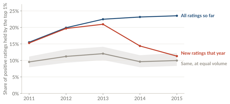
Counting all ratings received so far, the top 1% of users held 15.5% of positive ratings at the end of 2011 and 23.5% by 2015, and the rise also holds within the users present in 2011. The share of each year's new ratings seems to fall after 2013, but ratings collapsed from 11,138 to 929 a year. Redrawn to the same 743 ratings every year, 2013 and 2015 overlap: most of that fall is a volume effect.

Who receives the next rating?

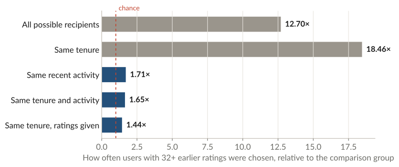
The standard way to measure preferential attachment from data (Barabási, Network Science, ch. 5) is to compare, for every new rating, the user who received it with everyone who could have. Users with 32 or more earlier ratings were chosen 12.7 times as often as chance, and the fitted rule \(\Pi(k) \propto k^{\alpha}\) has \(\alpha = 1.07\), almost exactly BA's linear attachment.

That compares a dormant newcomer with an active trader. Against users with the same tenure and recent activity the ratio falls to 1.65, and \(\alpha\) to a sublinear 0.68. Recent activity, not reputation, explains most of the advantage, and about half of all ratings simply return an earlier one, usually within minutes.

Robustness

Robust to failures, fragile to attacks

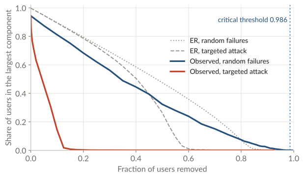
Percolation theory predicts when a network falls apart. A giant component exists while \(\kappa = \langle k^2\rangle / \langle k\rangle > 2\), the Molloy–Reed criterion, and removing a random fraction \(f\) of the users destroys it at the critical threshold

Random removal barely matters: the giant component survives until about 93% of users are gone. Removing the most-connected users first breaks it after 15%. Randomized networks with the same degrees break at the same point, so the hubs are the weak spot.

Drawn in Cytoscape

The most-rated users, close up

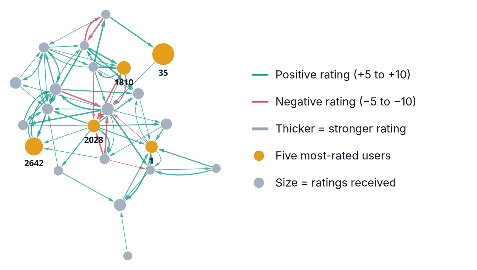
We also drew the 25 users with the most positive ratings and the strong ratings between them (±5 or more) in Cytoscape, and animated how those ratings appeared with CyAnimator. Three of the 25 have no strong rating with the others, so 22 are shown. Colour shows the sign of a rating, width its strength, and size how many ratings a user received.

The talk

The presentation

The fifteen slides of our thirteen-minute talk. Use the arrows, the arrow keys, or swipe; slide 9 plays the CyAnimator video. The arrow button (or a double click on a slide) shows them full screen.

Reproduce

Every number can be rebuilt

The repository has the analysis scripts, notebooks that work through each method by hand, the stored results, and a checker that compares a new run with the recorded one. With Python 3.12:

# set up the environment
python3.12 -m venv .venv
.venv/bin/python -m pip install -r requirements.txt
# put soc-sign-bitcoinotc.csv.gz from SNAP in data/, then
.venv/bin/python scripts/reproduce.py
.venv/bin/python scripts/verify_reproduction.py --check-manifest

See also the code walkthrough and the Cytoscape workflow.