


A real-time pipeline that watches 2,400 IoT devices for attacks and trains one shared detector from all of them. FLEAD streams the Edge-IIoTset network-traffic dataset through Kafka, scores every reading in Flink, trains a small model on each device, combines the device updates with differentially private federated averaging, evaluates every shared model in Spark and shows each stage live in Grafana and a monitor page.
It sets out to process a live IoT stream end to end with open-source tools, train one attack detector across thousands of devices from their model updates, measure detection on realistic labelled traffic, and make every stage visible while it runs.
The pipeline
From device files to live dashboards
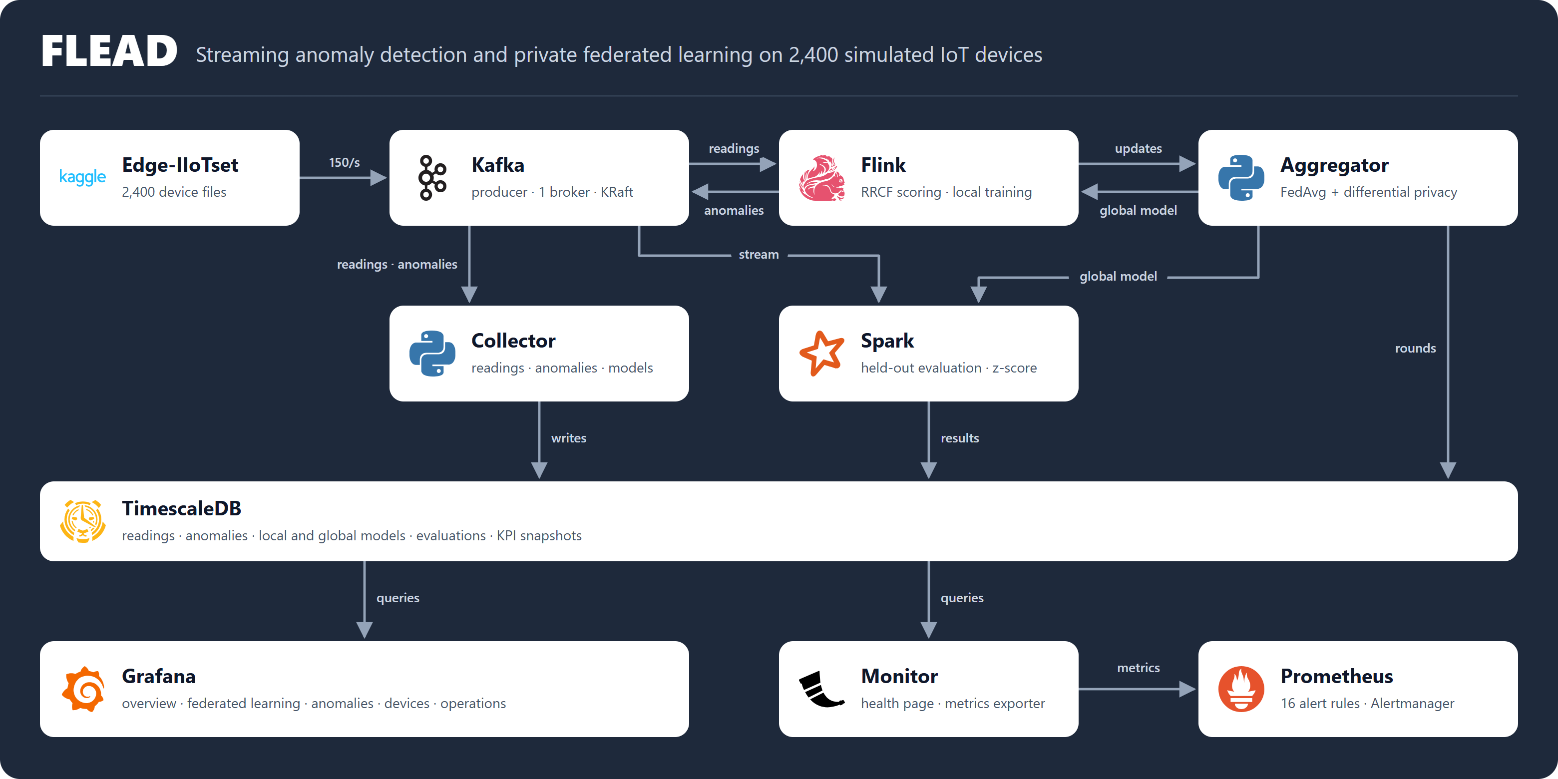
1  Data
Data
Edge-IIoTset’s 1,985,453 unique network flows, benign traffic and 14 attack types, keep 46 standardized features and are split at random into 2,400 device files.
2  Stream
Kafka’s producer replays every device at 150 readings/s. Each device streams its first 660 readings and keeps the other ~167 for testing.
3  Score and train
Flink scores each reading with a Random Cut Forest and retrains the device’s logistic regression after every 30 new readings.
4  Aggregate
Every minute the aggregator merges the latest device updates with DP-FedAvg into a new shared model for Flink and Spark.
5  Evaluate
Spark tests every shared model on held-out readings and compares each device with the rest of the fleet.
6 
 Store and monitor
TimescaleDB stores every stream and result; Grafana, the monitor page and Prometheus alerts show each stage as it runs.
Stream and batch
Two speeds of processing
FLEAD combines continuous stream processing, which reacts to each reading within seconds, with periodic batch processing, which summarises models and devices over longer spans. Both write to TimescaleDB, so the dashboards show them side by side.
Stream processing continuous, per reading
- Kafka carries readings, anomalies and model updates as keyed, ordered streams on four topics:
edge-iiot-stream,anomalies,local-model-updatesandglobal-model-updates. - Flink handles each reading as it arrives: it scores the reading with the forest, adds it to the device’s window and trains the device’s model after every 30 new readings.
- Spark Structured Streaming groups the live stream into 30-second event-time windows with a one-minute watermark and flags devices whose mean sits more than 3 standard deviations from the fleet.
- The collector writes readings, anomalies and local model updates to TimescaleDB as they arrive.
Batch processing periodic, over many readings
- Federated rounds run every 60 seconds over the latest update of each device, once at least 200 devices have reported.
- Held-out evaluation in Spark scores each new shared model over a cached sample of about 20,000 held-out readings, checking for a new version every 120 seconds.
- Device statistics in Spark compute the daily mean, standard deviation, minimum and maximum of every device’s stream metric from the device files.
- KPI snapshots summarise the whole fleet every 15 seconds: totals, active devices, anomaly rate and attack share.
The tools
What each tool does here
Apache Kafka
The backbone for real-time data: one broker in KRaft mode with four partitions per topic carries every stream between the services.
Chosen for a durable, partitioned log that several services read independently at their own pace, with keyed messages that keep each device’s readings in order.
Apache Flink
Runs the per-reading work, forest scoring and per-device training, on two parallel workers with the stream keyed by device id.
Chosen for stateful, low-latency stream processing: keyed streams send each device to the worker that holds its training window and model.
Apache Spark
Evaluates every shared model, analyses the live stream in windows and computes per-device statistics, on a master and worker cluster.
Chosen for one engine that covers both sides: Structured Streaming over Kafka and batch jobs over held-out readings and device files.
Python services
The federated aggregator (buffered FedAvg, differential privacy, model registry, update clustering), the Kafka-to-TimescaleDB collector, the KPI updater, and two Flask apps: the live monitor and the device viewer.
Chosen for direct control over the federated algorithm and privacy accounting, with NumPy for the model math.
TimescaleDB
Stores readings, anomalies, local and global models, evaluations, fleet windows, device statistics and KPI snapshots.
Chosen for PostgreSQL with hypertables that partition data by time: every service writes plain SQL, and recent data stays fast to query.
Grafana
Five dashboards over TimescaleDB and Prometheus: overview, federated learning, anomalies, devices and operations.
Chosen for rich time-series panels over SQL and PromQL, provisioned from dashboard JSON that FLEAD generates and tests in Python.
 Prometheus and Alertmanager
Scrape Flink, Spark and the monitor’s metrics exporter, evaluate 16 alert rules and send firing alerts to the monitor.
Chosen for pull-based metrics and rule-based alerting, with exporters that Flink and Spark provide.
 Docker Compose
Defines all services with health checks, startup order and shared volumes; START.bat and ./start bring the whole stack up and submit the Flink and Spark jobs.
Chosen for one command that runs the same stack on Windows, Linux and macOS.
Edge-IIoTset
The data source: labelled network traffic from IoT and industrial IoT devices, downloaded from Kaggle and preprocessed in its own container. Next to benign traffic it holds 14 attack types: DDoS floods over UDP, ICMP, TCP and HTTP, SQL injection, XSS, password attacks, uploading, backdoor, ransomware, man-in-the-middle, port scanning, vulnerability scanning and fingerprinting.
Chosen for realistic, labelled cyber-security traffic that stands in for private device data and lets both detectors be measured.
Design decisions
The ideas behind it
Decision 1 · anomaly detection
Random Cut Forest scoring
FLEAD scores every reading with a Robust Random Cut Forest. The forest learns one point at a time, adapts as the traffic changes and looks at all 46 features together, which suits many-dimensional network traffic. The fleet z-score in Spark adds a second view: each device against the rest of the fleet.
How a reading is scored. A random cut tree splits its points with random cuts, choosing each cut dimension in proportion to its range, so unusual points end up isolated near the root. A reading’s collusive displacement, how many points would move if it were removed, is its raw anomaly score.
- Insert the reading’s 46 standardized features into each of 4 trees; each tree keeps its 256 most recent points.
- Average the collusive displacement over the trees.
- Rank it among the last 500 raw scores: the score is 0 up to the 90th percentile and rises linearly to 1 at the top.
- Flag the reading when the score beats its device’s threshold. The threshold starts at 0.4 and moves by 0.02 every 50 readings to keep about 5% of the device’s readings flagged.
Choices that mattered. Using all 46 features of a reading raised ROC AUC from 0.51 with a single feature to 0.65–0.66. One shared forest per Flink worker compares every reading with current traffic across the fleet and keeps memory small. And 4 trees × 256 points gave the best precision of the sizes tested:
| Forest (60 devices, two samples) | ROC AUC | Readings flagged | Attacks among flagged |
|---|---|---|---|
| 1 × 256 | 0.54 / 0.55 | 6.0% / 5.9% | 62% / 60% |
| 2 × 256 | 0.55 / 0.60 | 6.3% / 6.0% | 44% / 54% |
| 4 × 256 | 0.65 / 0.66 | 6.1% / 6.0% | 86% / 81% |
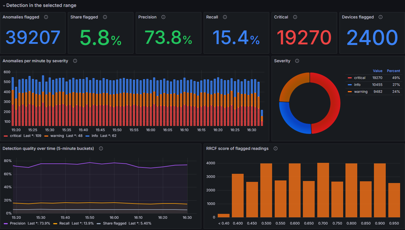
What it achieves. In the live run the forest flagged 5.8% of readings, and 74% of them were attacks against a 28% base rate: about 2.6 times the rate of random flagging. With a ROC AUC around 0.66 it is a strong ranking signal, and it works as a label-free early warning next to the federated classifier. Each flag carries its score, threshold, severity and the reading’s true label, so the dashboards show how many flags are real attacks.
Decision 2 · privacy
Private aggregation
The aggregator keeps each device’s latest update, its change since the global version it started from, and runs DP-FedAvg every minute:
\[ \Delta_i = w_i - w_{\text{base}(i)}, \qquad w_{\text{global}} \leftarrow w_{\text{global}} + \frac{1}{n}\sum_{i=1}^{n} \Delta_i \cdot \min\!\left(1, \frac{C}{\lVert \Delta_i \rVert}\right) + \mathcal{N}\!\left(0, \left(\frac{\sigma C}{n}\right)^{2}\right) \]
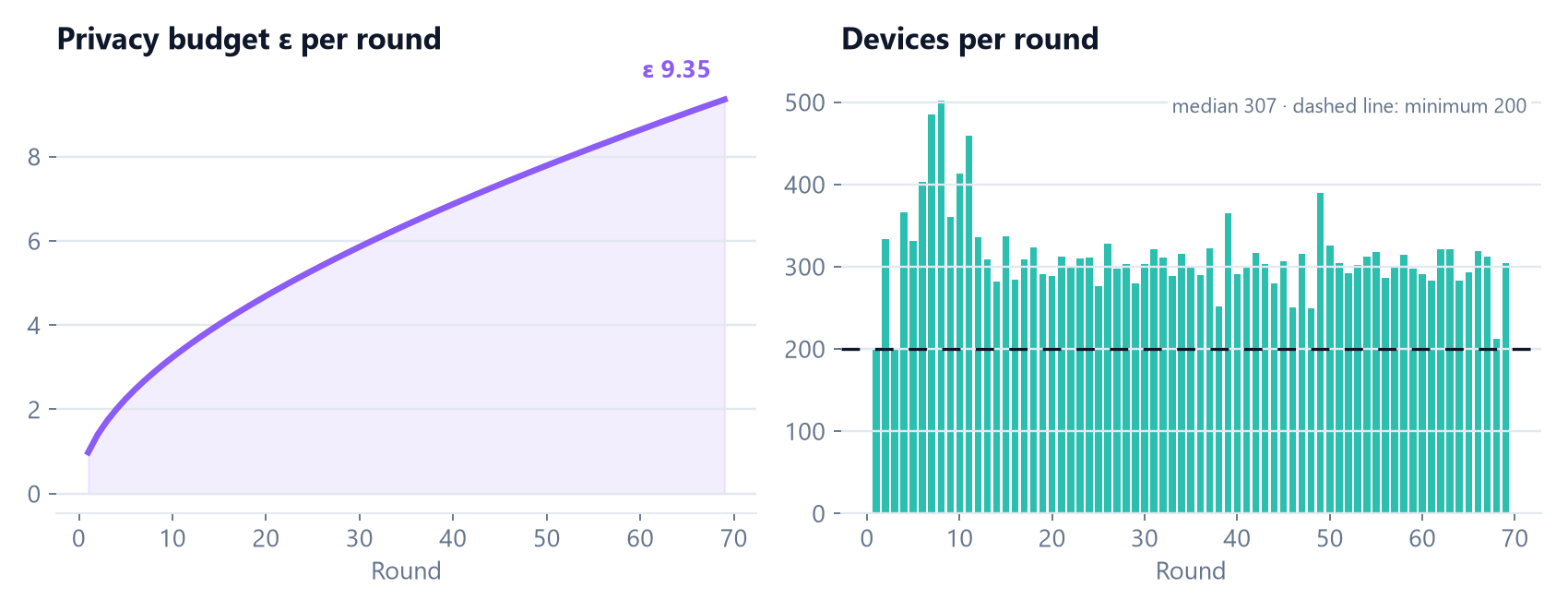
With clip norm \(C = 1\) and noise multiplier \(\sigma = 5\), every extra device lowers the noise. An offline run with 40 devices per round reached F1 0.58 against 0.73 with privacy off, which set the 200-device minimum. Live rounds with a median of 307 devices keep the noise around 0.016 while accuracy climbs from 0.770 to 0.875, and a Rényi-DP accountant tracks the budget: ε = 9.35 after 69 rounds. With privacy switched off, the average is weighted by each device’s sample count, as in classic FedAvg.
Decision 3 · evaluation
Scored on held-out readings
Every model version is scored on held-out readings with a full confusion matrix and shown next to the always-benign baseline. The same F1 drives the model registry, which republishes the best version whenever a newer one scores more than 0.10 lower.
Decision 4 · streaming pace
Training at the pace of the stream
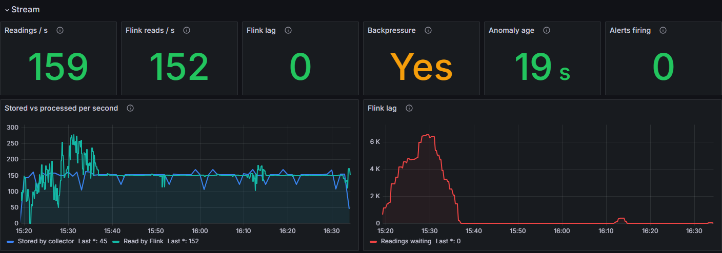
Local training runs after every 30 new readings of a device, which keeps Flink at the full 150 readings/s. A per-device offset from a hash of the device id spreads training evenly, so federated rounds arrive about once a minute.
Results
What one run showed
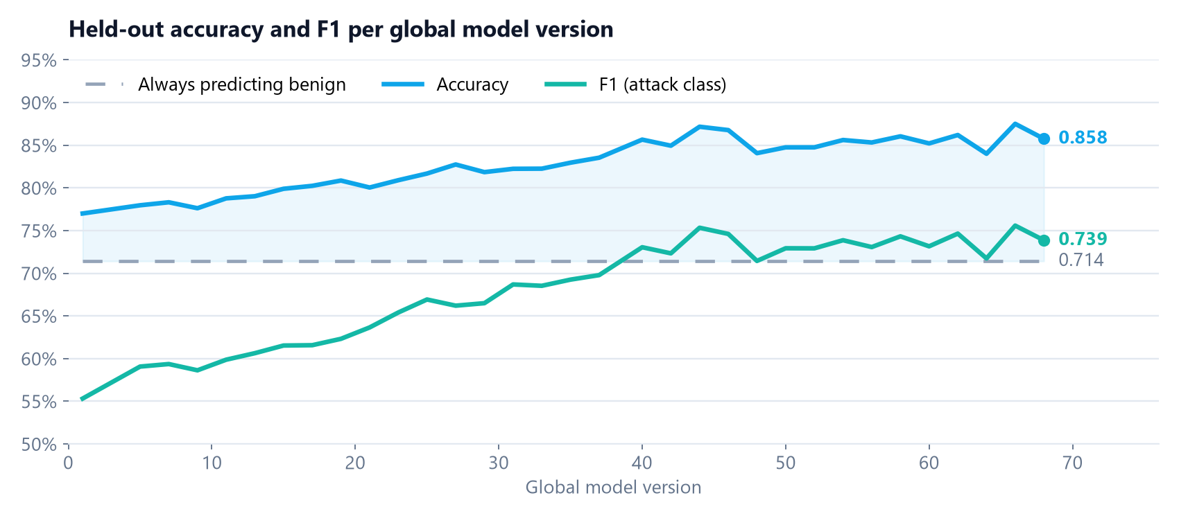
One 77-minute run of the full pipeline. Held-out accuracy and F1 rise steadily as rounds add device updates and the shared model settles.
0.84–0.875 held-out accuracy over the last 10 rounds (baseline 0.714)
0.72–0.76 held-out F1 for attacks over the last 10 rounds
74% of flagged readings are attacks (base rate 28%)
150/s readings streamed, 694,999 of 695,000 confirmed
| Metric | Result |
|---|---|
| Held-out accuracy / F1 | 0.770 / 0.553 after round 1; 0.840–0.875 / 0.717–0.756 over the last 10 evaluations (rounds 50–68); 0.858 / 0.739 at round 68 |
| Precision / recall (round 68) | 0.777 / 0.704 on 19,981 held-out readings |
| Always-benign baseline | 0.714 |
| Federated rounds | 69, median 307 devices per round (200–502) |
| Privacy | ε = 9.35 after 69 rounds (δ = 10⁻⁵), median noise σ 0.016 |
| Anomaly scoring | 5.8% of readings flagged, 74% of them attacks |
| Stream | 150 readings/s; 694,999 of 695,000 readings confirmed by Kafka |
Interfaces
See it running
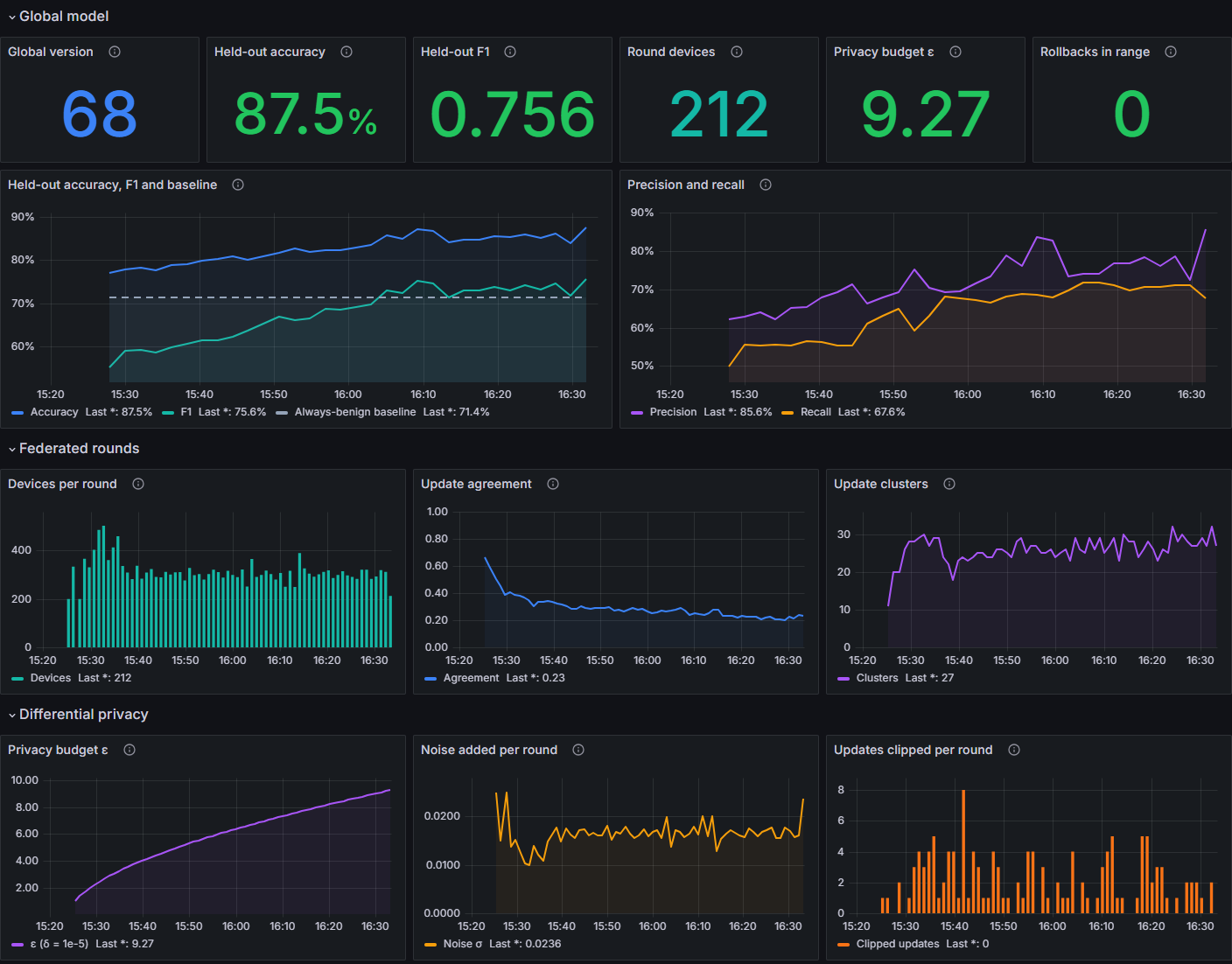
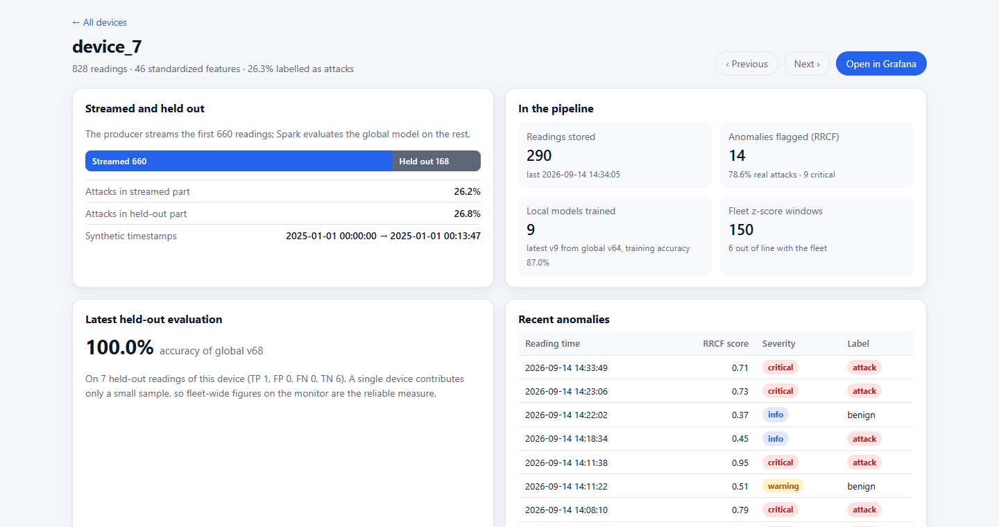
The live monitor during the run: overall status, model quality, privacy budget, latest round and Flink lag.
Scope
Scope and next steps
Scope
- Simulated fleet: devices are random slices of one dataset, and every reading also flows through Kafka and the database for measurement.
- One Kafka broker.
- Logistic regression as the classifier.
- Privacy protects each update as seen through the shared models, with a conservative ε.
Next steps
- LSTM or GRU sequence models on each device’s stream.
- Kubernetes deployment for scaling out and self-healing.
- Real IoT and edge devices in place of the dataset replay.
- A replicated multi-broker Kafka cluster.
Try it
Run it yourself
START.bat     # Windows
./start       # Linux, macOS
Needs Docker with about 8 GB of memory and a Kaggle API token for the dataset. Once the pipeline is up, the script opens the monitor (http://localhost:5001) and Grafana (http://localhost:3001). The 53 unit tests run on their own with pytest tests.
Credits
Data: Edge-IIoTset (Ferrag et al., 2022). Algorithms: Robust Random Cut Forest (Guha et al., 2016), FedAvg (McMahan et al., 2017), DP-FedAvg (McMahan et al., 2018), buffered asynchronous aggregation (Nguyen et al., 2022), Rényi differential privacy (Mironov, 2017). Early prototype: github.com/suu00k1459/OST.